Simple neural network
Maciej Mazurek , 20 January 2020

Introduction
The purpose of this article is to present the concept of neural networks, specifically the feedforward neural network, by constructing a simple example of such a network in Python.
The neural network is a statistical computational model used in machine learning. You can think of it as a system of neurons connected by synapses that send impulses (data) between them. The neural network consists of three layers: the Input Layer, the Hidden Layer, and the Output Layer, as illustrated in Diagram 1.
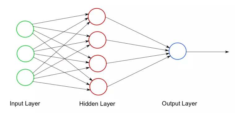
The input layer accepts input for calculations. All calculations take place in the hidden layer. The result of these calculations is sent to the output layer.
In the diagram above, the circles represent neurons and the arrows represent synapses. Each synapse has a weight, i.e. a number that determines "how strongly the transmitted value affects" the final result of the calculation. To send a value, the synapse first reads the value from the input neuron, then multiplies the value by weight and sends the result to the output neuron. Then the output neuron performs calculations on the values provided by the synapse and passes the result to the outgoing synapse.
Training the neural network is a process whose goal is to select appropriate weights for synapses. We assume that how the calculations inside each neuron are made is invariable. Training is an iterative process. One iteration consists of two (performed in the given order) steps: forward propagation and backward propagation.
The forward propagation consists of performing calculations on the input data using weights assigned to synapses. Backward propagation measures the error of the forward propagation result (by comparing it with the expected calculation results, i.e. with training data). Depending on the measured error, synapse weights are modified (it can be said that by adjusting the weights the network "learns from its errors").
Example
This section will demonstrate how to construct a simple neural network that implements the concepts described in the introduction.
Consider the following problem. The three bit long binary number is given. We want to determine if this number is even or not. Below are some examples of input data along with the expected values at the output.
| Input value | Expected result |
| 101 | 0 |
| 110 | 1 |
| 010 | 0 |
The above table is a symbolic set of training data. Each input value is assigned to the expected calculation result.
Neural network structure
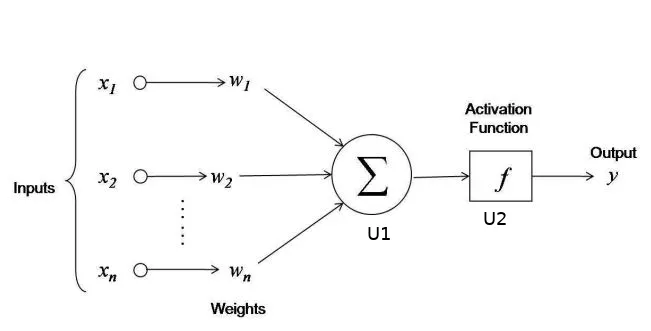
Diagram 2 presents the structure of our neural network. The input layer consists of three neurons (each neuron corresponds to a single bit value of the binary number from the input). The hidden layer consists of two neurons: U1 and U2. Neuron U1 sums up all the numbers it received, with appropriate weights, and then transfers this sum to the neuron U2. The weight of the synapse from neuron U1 to neuron U2 is 1 (if the weight is not specified, its default value is 1). Then the neuron U2 imposes an activation function on the result of the calculations made in the U1 neuron (which will be described in detail in the later text) and passes the result (again with a weight of 1) to the output layer.
Forward propagation
From what has been said above, it is clear that the weights must have a predetermined value when forward propagation is first performed. Each of them will be initiated with a randomly selected number from the range (-1, 1). However those values need to satisfy one condition. The expected value of the weights (for some theoretical reasons, which we omit here) must be 0.
Forward propagation is carried out as follows. First, neurons from the input layer are initialized with the bits of the input number. Then the value of each neuron from the input layer is multiplied by the appropriate weight and is sent to the neuron U1. Neuron U1 sums up all three values.
The result calculated in the neuron U1 still needs to be "interpreted". The U1 value can be thought of as a measurement of dispersion. For example, if we get the number 332482 in the neuron U1, then our neural network claims that the correct result is very likely (almost sure) to be 1. If the neuron U1 calculated the number -54387, our network predicts that the correct result is 0. If instead neuron U1 has calculated a value of 0, our neural network has no idea what the correct answer is (or even could be).
The interpretation mentioned above takes place in the U2 neuron by using the appropriate activation function. There are many different models that use various activation functions. For our purposes, the best is the sigmoid function, the graph of which is presented in the figure below.
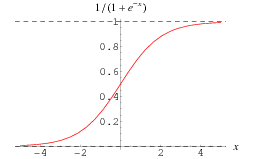
It can be seen that this function "interprets" the calculation result from the neuron U1 as expected. For large inputs function outputs are close to 1, for small - close to 0. Note that for the argument 0 the sigmoid function yields the value of 0.5.
Backward propagation
Suppose we perform one iteration of the training process for a pair (110, 1) - the first value from the tupple is the input data, the second is the expected result. Let us denote by R the calculated value in the neuron U2 for the input data described above during forward propagation.
We will start backward propagation by calculating how much the value calculated during forward propagation differs from the expected result.
error = R - expected_resultThen - depending on the error received - we need to improve the weight of synapses. In the method used in this example, the optimization of a single weight is as follows.
error = R - expected_result
weight = weight + expected_result * error * d_sigmoid(R)
where d_sigmoid (R) is a derivative of the sigmoid function at x = R. If the reader is interested in the genesis of the above formula, please refer to https://en.wikipedia.org/wiki/Logistic_regression. As an indication, the error measuring function is a convex function, so it can be minimized by going "along its gradient" - that is, towards its global minimum.
The code
import numpy as np


class SimpleNeuralNetwork:
    """
    Simple neural network that checks if a given binary representation of a positive number is even
    """

    def __init__(self):
        np.random.seed(1)
        self.weights = 2 * np.random.random((3, 1)) - 1

    def sigmoid(self, x):
        """
        Sigmmoid function - smooth function that maps any number to a number from 0 to 1
        """
        return 1 / (1 + np.exp(-x))

    def d_sigmoid(self, x):
        """
        Derivative of sigmoid function
        """
        return x * (1 - x)

    def train(self, train_input, train_output, train_iters):
        for _ in range(train_iters):
            propagation_result = self.propagation(train_input)
            self.backward_propagation(
                propagation_result, train_input, train_output)

    def propagation(self, inputs):
        """
        Propagation process
        """
        return self.sigmoid(np.dot(inputs.astype(float), self.weights))

    def backward_propagation(self, propagation_result, train_input, train_output):
        """
        Backward propagation process
        """
        error = train_output - propagation_result
        self.weights += np.dot(
            train_input.T, error * self.d_sigmoid(propagation_result)
        )
Explanation
Finally, we will explain how the above Python class implements the described concept (we assume that the reader knows the basics of Python).
In the SimpleNeuralNetwork class initiator, we first "initialize" a random number generator (line 9), and then specify the initial weight values as a three dimensional column vector filled with random numbers (line 11). For details, refer to the numpy documentation.
The forward_propagation function is responsible for carrying out the forward propagation process. Input data (three bits of a binary number) are passed to this function as a three dimensional vector. The following code
np.dot(inputs.astype(float), self.weights)calculates the scalar product of the weight vector and the input vector. By passing this value to the sigmoid function, we get what we want.
The backward_propagation function implements the backward propagation process. First, the error is calculated relative to the expected result (line 41). Then synapse weights are modified. Code
self.weights += np.dot(
    train_input.T, error * self.d_sigmoid(propagation_result)
)
performs the previously described calculations on each coordinate of the weights vector. The np.dot is the matrix multiplication,train_input.T is transposed train_input matrix.
Testing program
network = SimpleNeuralNetwork()

print(network.weights)

train_inputs = np.array(
    [[1, 1, 0], [1, 1, 1], [1, 1, 0], [1, 0, 0], [0, 1, 1], [0, 1, 0], ]
)

train_outputs = np.array([[0, 1, 0, 0, 1, 0]]).T

train_iterations = 50000

network.train(train_inputs, train_outputs, train_iterations)

print(network.weights)

print("Testing the data")
test_data = np.array([[1, 1, 1], [1, 0, 0], [0, 1, 1], [0, 1, 0], ])

for data in test_data:
    print(f"Result for {data} is:")
    print(network.propagation(data))